Circular Reference Warning-
Sometime you get Circular Reference Warning when you open Excel document. Though you can simply press OK and but recommend you not to ignore such warning as there are some calculation errors in your sheet.

We have to remove Circular Reference Warning to get perfect result in Excel file.
Why Circular Reference Warning display??
Circular Reference Warning display when formula cell itself include in formula. Means if you type formula in A1 – A1 + B1 then excel display this warning. You should identify and remove warning because the wrong answer display by formula. Generally you get answer zero if any Circular Reference use in formula. Each time when you open file you’ll get Circular Reference Warning until you resolve them.
How to remove Circular Reference Warning display??
To find the cell where circular reference added go to Formula tab and click on drop down of Error Checking option and choose third option Circular References.

In Circular References option you can find cell address where error occurred. Simply click on that cell reference. Excel automatically goes to that cell.
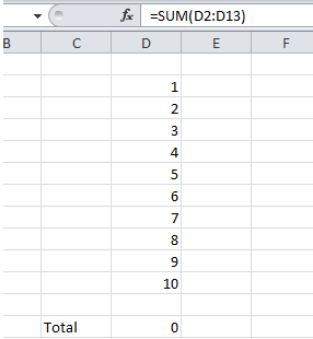
On above screenshot total of all numbers should not be zero but because of Circular References it shows answer zero.
Once you click on cell address from circular option cursor automatically goes to that cell. Now check formula and remove the Circular References cell from formula. It may be include in Range which use in formula or may be only cell.

Click again on Error Checking button from Formula tab and resolve all Circular Reference cell until option of Circular Reference change to grey or unclickable.
Now save and close the file. The Warning Circular Reference will not show any more.
Watch Video -
Hope you understand
Thank you. Have a nice day. Enjoy Excelling..
No comments:
Post a Comment