How to Hide all Formulas in Excel in Just 2 Steps

Hide all Formulas in Excel

Sometime you want to share your excel files but you don’t want to share formulas in that excel files. You want to hide particular or all formulas in Excel.

You can hide all formulas in sheet easily. There are two main steps to hide formulas in Excel.

Lets Start –

By Default protection of all cells are Locked and not hidden. But this only work when sheet is protected. Lets understand how it matters.

First Step to hide formula is to change Format of those cells which contain formulas.

To Change Format select all cells in sheet with Ctrl + A and Go to format cell with Right Click. Untick Locked option

Then to hide cells formula and locked cells which contain formula we have to change protection of those particular cells.

To select Formula Cells click on Special option from go to with F5 key or Ctrl + G.

Select Formulas from Go To Special and click on OK. You can see only cells which contains formula are selected.

Now Right Click and Choose option Format Cell. And from Protection Tab tick on both options Locked and Hidden.

 

Now Second and Last step is  to protect Sheet. To protect sheet go to Review Tab and Click on Protect Sheet.

You can set password for sheet and also change rules as per your requirement. This will apply only for cells which contain formulas. Then click on Ok.

Now you can see formulas is not shown also when you try to edit formula then excel will display below Warning.

Hope you understand how to hide all Formulas in Excel

Thank You.

Watch Video -

Have a nice Day...Enjoy Exceling..

Hide cell value only without hiding Row and column - quick tips

Hide cell value only without hiding Row and column

Sometimes you want to hide cell value only and not any row or any column. But that hidden value can be used in any formula without any issue.

To hide only cell values first select that particular cell.

Then right click on it and select option Custom from Format Cells

Then in Type field enter three times semicolon (;;;) same as highlighted in below screenshot and hit Ok.

Now you can see cell value is hidden but it is not affected formula and also note it is display only in Insert Formula Bar.

Hope you understand as it is very easy

Watch video

Thank you…Enjoy Excelling

Fill color in every alternate row in Excel - Shortcut

In this tutorial I’ll show you how to fill color in every alternate row in Excel or how to highlight every alternate row in Excel.

If you have small data and you want highlight or fill color in every alternate row then it take less time to do manually. But what if you have more than hundreds or thousands of row then it will be very time consuming. Thus in this post I’ll show you how to highlight every alternate row easily and that too without consuming much time.

Lets Start -

We are going to use Conditional formatting Rule to highlight alternate Row.

First select all Data then go to Conditional Formatting and select New Rule.

We have to create new Formatting rule. Select a last Rule Type “Use a formula to determine which cells to format” and in Edit the Rule Description field type formula “=mod(row(),2)”.

After typing formula click on Format button and select format which you want. Here I have select Bold Font and Fill Orange Color in Format Cells window.

Then click on Ok button. Now you can see all alternate row change in format you choose.

Hope you understand how to Fill color in every alternate row in Excel.

If you have any issue then feel free to comment on Post.

Have a nice day…. Enjoy Excelling …..

Restrict duplicate entries while entering new values in Excel

Sometime you don’t want duplicate entries in your list which you prepare in Excel. There is easy fix to restrict duplicate entries while entering new values. Just follow up below process and you will see error occurred when you try to enter duplicate values in range.

Lets Start -

First Go to Data tab and select first option Data Validation from Data validation menu.

Then below Window will open.

In Allow option select dropdown and choose Custom and enter CountIf formula in Formula Field.

Countif formula should be like as per above. It should include Range where you want to enter data with fixed Reference by putting $ sign in Cell Reference. Shortcut for lock Range is select Range and press F4 Key. Then also put “ =1 ” to enter value in Range only once.

Then click Ok.

After that Drag that Cell till Last Cell in Range. Here I have dragged D5 till D20.

Now you can see below error when you try to enter same value again in Range.

Note – Data Validation will not work if you copy paste value from other location.

You can customize above error message. To customize your own error message go to Data Validation and select Error Alert tab.

Enter Title and Error message what you want to display while entering duplicate values.

Hope you understand how to restrict duplicate entries in Range.

Thank you

Watch Video -

Have a nice day….Enjoy Excelling…

Send whole email from Excel without using Macros

In this post you will learn how to send whole email from Excel without using Macros.

You may know you can send email from excel with using VBA Macros but it is not so easy to understand everyone. Today I’ll show you how to send email from Excel without using Macros. We can send whole email from Excel by using just formula.

Lets Start –

Before starting tutorial make sure you should configure outlook in PC otherwise it won’t work.

I have written subject, CC and email body in column A and B as per below.

To send this email particular person we want link to click and auto create mail in Outlook. To Generate link, we are using HYPERLINK formula.

Now enter Name and Email List in Column A and B below or side of above Mail.

From above data and HYPERLINK formula we are going to generate link which help to create email directly in Outlook.

Formula is looking too big but it is very easy to understand.

Lets Understand Formula and Criteria –

 Hyperlink is required Two Criteria

1.       Link Location – Our Link location is as per below -

mailto – Select Cell where you have person’s Email ID. Here - B11

CC – If you have CC in your mail then select that cells. Here – B2

Subject – Select cell where subject appear. Here B3

Body – Body may contains multiple and blank lines so we are using “%OA” for next line and blank cell for blank lines

               

2.       Friendly Name – You can use any name for above Link which will appear in cell where you enter formula with link.

Make sure you have lock all the cells which use in CC, subject and Body as we are not changing any field. We are only change receiver email id.

Now you get link with Friendly Name. Here send e-mail.

Just Click on Link and you can see Excel will redirect to Outlook with whole email.

Now you are ready to send email from Excel without using Macros.

Note – As Hyperlink only support up to 256 characters so you won’t be able to large mails.

To Download above Template click on Link below –

Download Template 

Hope you understand how to Send whole email from Excel without using Macros 

If you have any issue then feel free to comments on Post.

Thank you

Watch Video - 

 Have a nice Day…. Enjoy Excelling……

Excel Copy Paste Multiple Values only in Blank cells - Shortcut

Excel Copy Paste Multiple Values only in Blank cells

If you have list with blank cells and you want to paste some data in blank cells only without changing other cells then follow below process.

Below I have written few numbers with blank cells and I want to paste remaining numbers in blank cells.

I have also remaining number in other column like below.

If we copy above range and paste into first image then it will give us same data display in 2^nd image. But we don’t want same data. We want to copy above data and paste it into blank cells only.

To copy and paste into blank cells only follow below process. It is very easy.

First Copy the Range you want to paste it. Here Range in column J. Then come to column D1 and Right click and select option Paste Special.

In Paste Special – Select Option Values and check mark on Skip blanks. Then press OK. Now you can see numbers only paste in blank cells an all other cells remain same as per below.

Hope you understand. If you have any issue then feel free to comment.

Thank you

Watch Video -  

Have a nice Day…Enjoy Exceling….

Excel Move Data from Column to Row and Vice-versa - Easy Trick

Excel Move Data from Column to Row and Vice-versa 

If you have data in horizontal format and you want to move the same in vertical format or vice-versa, in other words you want to move data from column to row or vice-versa then follow below simple steps.

It is very easy to follow below steps rather than enter them manually.

In above image you can see date is in horizontal format in column but we want to transfer them in vertical format in Row then copy data and select any cell where you want data.

Right click and select option Paste special then tick on transpose option. After Tick on transpose option hit on OK.

Now you can see all values are transfer to vertical format in Rows.

Hope you understand how to Excel Move Data from Column to Row and Vice-versa.

Thank you.

Watch Video -

Have a nice Day… Enjoy Excelling…

How to break password of protected sheet in Excel without any software – In 30 seconds

Break password of protected sheet in Excel without any software

There may be chances that you forget password of protected sheet or you want to remove password of protected to enable edit. You can’t edit sheet if same is protected and if you try to edit then below warning pop up display.

 

So this post is for those people who want remove password of protected sheet & transfer protected sheet from unprotected sheet and that too without any software.

Lets Start 

1. Change file extinction to zip

If you can view extension of file then you can change it to zip easily. In case you are not viewing extension then follow below steps

A. Click on Start

B. Type Folder Option in search box

 

C. Open Folder option

D.   Untick on Hide extension for Known file types

 

Now you can able to see file extension and change it to zip

2.  Edit file

Open zip folder and copy sheet 1 (your sheet name may be different ) from worksheet folder and paste the same in outside zip folder

Open that sheet with Notepad by right click and open with option.

 

Then delete sheetProtection tag and save the file

<sheetProtection password="C746" sheet="1" objects="1" scenarios="1"/><pageMargins left="0.7" right="0.7" top="0.75" bottom="0.75" header="0.3" footer="0.3"/>

3. Replace file

Replace this new file with old one in worksheet folder.

4. Change file extension to xlsx again

Now the last step is to change zip folder extension again to xlsx and open the file. You can now able to edit the sheet and no more password restriction for sheet.

Hope you understand

Watch Video

Thank you..Enjoy Excelling…Have a nice day..

Comparison Between Index Match and Vlookup Formulas in Excel

Comparison Between Index Match and Vlookup

There two most powerful lookup formulas in excel. First one is Vlookup and second one is Index Match. Vlookup is most common formula nowdays and it is very much popular in Excel. On the other hand Index Match is not so popular but it works same as Vlookup. In fact Index Match is two different formulas Index and Match which combine to get result of lookup. In this post we compare both formulas with different criteria to understand which one is need to be used.

Lets Start -

1. Easy to Understand - 

Most of the people understand Vlookup is very easy as compare to Index Match. Index Match is more large formula compare to Vlookup and it has include two ranges so user may confuse which range to use.

Syntax of Vlookup - 

=VLOOKUP(lookup value, range containing the lookup value, the column 
number in the range containing the return value, 0) 

 Syntax of Index Match -  

=INDEX (column to return a value from, MATCH (lookup value, column to lookup against, 0)) 

Thus most of the people use Vlookup formula as they may be think Index Match is difficult to remember or they don't aware about index match function.


2. Delete / Insert Column - 

There may be chances that you want to delete or insert extra column in sheet after completing sheet.
If in that sheet vlookup formula is included then after deleting or inserting column that formula has #REF reference error.
But it is not the case in Index Match Formula. You can delete or insert column which is not used in formula iteself but formula works fine.
So Index Match is better than vlookup to avoid errors in future. 

3. Right to Left - 

Vlookup only works in one direction i.e. left to Right. If suppose column to return value from is at left side from column to lookup against then vlookup not works. We have to copy paste that column at right side then we can use it.
But in Index Match it dosen't matter which column is on which side. It works perfectly without any condition. We don't want to adjust data to use Index Match formula.


4. Array

Vlookup is not consist array range. We have to adjust data by adding extra column and by using other formula to get result.
Index Match can be use with array. It works perfectly when we have multiple criteria.

 Syntax of Index Match with multiple criteria -  

{=INDEX(range1,MATCH(1,(Lookup Value1=Lookup range1)*(Lookup Value2=Lookup range2),0))}

 Ctrl + Shift + Enter to complete Array Formula

Conclusion - 

Though Vlookup is more popular than Index Match formula but the fact is Index Match is better and more powerful lookup formula than vlookup. Thus forget Vlookup and start to use
Index Match. 

Please watch video tutorial to understand in better way

Thank you..!! Enjoy Excelling !!

Have a great day !! 

How to Remove Circular Reference Warning in Excel ?

Circular Reference Warning-

Sometime you get Circular Reference Warning when you open Excel document. Though you can simply press OK and but recommend you not to ignore such warning as there are some calculation errors in your sheet.

We have to remove Circular Reference Warning to get perfect result in Excel file.

Why Circular Reference Warning display??

Circular Reference Warning display when formula cell itself include in formula. Means if you type formula in A1 – A1 + B1 then excel display this warning. You should identify and remove warning because the wrong answer display by formula. Generally you get answer zero if any Circular Reference use in formula. Each time when you open file you’ll get Circular Reference Warning until you resolve them.

How to remove Circular Reference Warning display??

To find the cell where circular reference added go to Formula tab and click on drop down of Error Checking option and choose third option Circular References.

In Circular References option you can find cell address where error occurred. Simply click on that cell reference. Excel automatically goes to that cell.

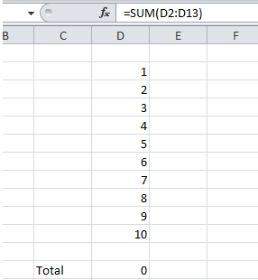
On above screenshot total of all numbers should not be zero but because of Circular References it shows answer zero.

Once you click on cell address from circular option cursor automatically goes to that cell. Now check formula and remove the Circular References cell from formula. It may be include in Range which use in formula or may be only cell.

Click again on Error Checking button from Formula tab and resolve all Circular Reference cell until option of Circular Reference change to grey or unclickable.

Now save and close the file. The Warning Circular Reference will not show any more.


Watch Video - 

Hope you understand

Thank you. Have a nice day. Enjoy Excelling..

Formula Error in Excel - You should Know

Excel formula help you to do lengthy calculation easily but for that you should know exact formula.
Arguments which use in formula should be correct to get correct answer. If we type wrong formula or argument then we get wrong answer and most probably ERROR.

There are mainly four types are error occur when we type wrong formula -

Lets understand how error comes and what we need to do to resolve them.


1. #VALUE!  ERROR

Value error occurred when formula has wrong type of argument means when you want total
of numbers but text is included in number then excel displays Value error.

Error

Solution

Solution – Simply remove wrong argument from formula.

2. #DIV/0! ERROR

DIV error displays when you divided any cell or number with 0. This is simple math rule. You can not divide any number with zero.

Error

Solution

 Solution - Change zero to another number

3. #REF! ERROR

REF errors displays when excel unable to find cell reference. Generally this error displays when
you deleted some row / column from sheet which used in formula.

Error

Solution

Solution – Remove #REF! from formula and / or add proper reference in formula.

4. #NAME? ERROR

NAME error displays when excel does not recognize text in formula. If you have mentioned
wrong range name or function name is incorrect then NAME error occurred.

Wrong name range -

Error

Solution

Wrong function - 

 

Error

Solution

Solution - Correct formula or remove unrecognized text from formula

Hope you understand. Feel free to comment if you have any doubt.

Watch Video - 

Thank you. Have a nice day. Enjoy Excelling